Chromatic Confessions of Salt Stressed Plants: AI to Read Between the Leaves
Uncover how machine learning can be used to spot salt stress in plants, revolutionising how we farm amidst sea level rise.
Published on 3rd July 2025
Stop, that’s A-salt!
Salt and plants have a complicated relationship. Too little salt and essential nutrients struggle to be absorbed. Too much salt? For plants without adaptations this means botanical Armageddon, as cell membranes break down. As a result of climate change, rising sea levels and altered rainfall patterns will modify soil salinity, causing significant shifts in vital ecosystem services such as nutrient cycling and food production. These effects will be felt strongly in estuarine and seafront locations, allowing readers to examine their summer holiday geographies in a new light (Figure 1).

Figure 1: Beach Day with a side of science. Next time you're relaxing at the coast, take a closer look at the plants around you. Shoreline botanicals face the front lines of rising seas and changing rainfall, quietly dealing with increasing salt levels in their soils. Applying survival strategies not sun cream: these holiday spots are perfect places to see climate change in action, if you know what to look for.
Monitoring helps drive adaptation, but lab-based methods come with a drawback—one tends to need a lab. Salt intrusion’s global threat necessitates a low-cost, easily deployable solution; a solution potentially arrived at by Del Cioppo and team in their recent publication in the Botanical Journal of the Linnean Society. Their machine learning (ML) approach was based around transparency and digital photography, generalising well to non-model species (species the model was not trained on).
They set out to:
- Examine the performance of ARADEEPOSIS (a publicly available model) at deriving quantitative phenotypes from studied plants.
- Identify key phenotypic traits expressed in plants to be used as stress markers.
- Test an integrated pipeline, combining image analysis (both human and machine) with minimal laboratory analysis.
- Build a classification model able to predict (1) stress occurrence and (2) intensity.
Machine Learning (ML) approaches
Neural Networks (NNs) have been all the rage recently. The cool kid on the block, NNs can catch non-linear relationships in data. However, they are computational “black boxes”; researchers have to play digital detective to find how they classify, e.g. which bee species visited a flower?
Appropriately for a plant related paper, the team used “Decision Tree” based models instead (Figure 2). These ML models allow one to examine the exact traits selected for classification, are computationally cheap and work well with small datasets. Del Cioppo et al. used 90 plants in total, so chose well for the dataset size.
Figure 2: This is not a figure of decision trees, but handy to imagine what they do. The point at which each branch splits is a decision point, determining if a particular feature is used in the model. The tips of the branches—the leaves—represent different classification conclusions such as "Stressed" or "Not Stressed." By following data along the decision points, you can classify data. Much like a forest ecosystem, multiple decision trees working together (in methods like Random Forest) can create more robust predictions than a single tree working alone.
The three pipeline stages
Machine Learning is a tripartite process (Figure 3), beginning with phase 1: data collection and analysis. Two plant species were selected for this experiment: the model organism Arabidopsis thaliana and the non-model Phaesolus vulgaris (Common Bean). The Common Bean plants were from two distinct varieties (FDL and FDA), to better understand crop response across strains. The plants were irrigated with varying saline solutions; some with standard “tap water”, some with moderate salt stress, while others received the solution equivalent of human tears. Top-down photos of the plants allowed image analysis (both manual and automatic), while physical samples were sent to the laboratory. This provided traits such as leaf green/yellow area or chlorosis (percentage of yellow area) for study, alongside traits such as relative water content (RWC) and Proline (an amino acid stress indicator) content.
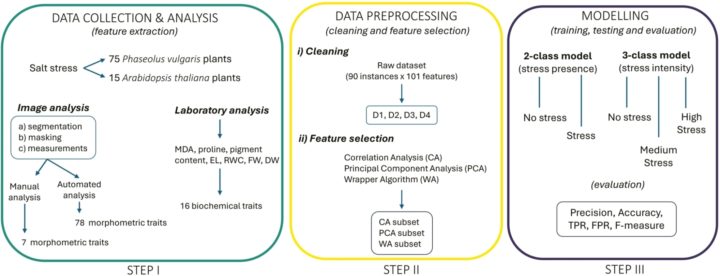
Figure 3: Machine Learning Workflow. The scheme illustrates the whole workflow followed. It starts with data collection and analysis (STEP I), which leads to feature extraction. It goes on with data pre-processing, which includes data cleaning and feature selection (STEP II), and ends with the modelling step (STEP III), which comprises training, testing, and evaluation of the machine learning models applied. MDA: malondialdehyde; EL: electrolyte leakage; RWC: relative water content; FW: fresh weight; DW: dry weight; TPR: true positives rate; FPR: false positives rate.
The next step in a ML pipeline is data pre-processing—cleaning datasets to then select the traits models will be trained on. Providing too many features can confound training, confusing the models and increasing the time taken to train them, so trimming the number of features is vital. Del Coppio et al. used three methods to get three data sub-sets, ready for the final stage.
The third and final part is model training, testing and evaluation. The light at the end of the pipeline, the brain in the machine (though it’s unsure what they dream about). A variety of models were trained along two threads. Firstly, stress presence/absence—literally asking if there is an abiotic stress? Secondly, is there an intermediate level? This model took aim at three levels of classification, instead of the binary first model.
A tale of two species
The results revealed an unexpected plot twist. Arabidopsis followed the conventional stress script; chlorophyll decreased while leaf yellowing increased. The Common Bean, however? Under severe stress, the FDA population saw a 2.5-fold increase in chlorophyll! Under severe stress, chlorophyll content increased. To vindicate Del Coppio et al. studying two bean populations, both displayed dramatically different biochemical responses to salt stress. FDA showed proline concentrations 13 times higher than control plants, while FDL increased just 2.7-fold. Malondialdehyde content (MDA), a key oxidative stress marker, followed a similar pattern, with stressed FDA showing levels 2.5 times higher than stressed FDL.
These species-specific and population-specific responses highlight why universal stress detection is so challenging—different plants quite literally speak different biochemical languages when stressed.
Plants and their technicolor dreamcoat
The most valuable discovery? Certain colour features, particularly "Chroma Difference" and "Chroma Ratio," proved to be reliable digital equivalents of these biochemical signals. This allowed the dropping of biochemical features, in favour of image derived traits. But what are these mysterious indices?
When a digital image is analysed, each pixel contains three colour values: red, green, and blue (RGB). Chroma indices combine these values, revealing subtle colour patterns invisible to the naked eye. "Chroma Difference" measures the gap between the dominant and weakest colour channels, capturing how "pure" or "diluted" a colour appears. "Chroma Ratio," meanwhile, calculates the proportion between colour intensities, revealing shifts in colour balance.
It turns out plantae broadcast their internal biochemical states in technicolour (Figure 4), we just needed the right decoder.

Figure 4: Hidden in plain sight: bees see UV flower patterns invisible to humans. Now, like discovering a new colour, chroma ratios let scientists spot the stress signals plants have been broadcasting all along. One up for humanity!
Performance beyond precision
The results of trained models weren't just good—they were remarkably impressive. The 2-class model (stress presence/absence) achieved 91 % mean precision with the most performant dataset, but the real story lies beyond this headline number.
Perhaps most critical for agricultural applications is avoiding false negatives. Did the models classify stressed plants incorrectly? The resounding answer was NO.
An exceptional True Positive Rate (TPR) of 0.967 for stress detection was achieved—meaning it correctly identified nearly 97 % of stressed plants. In practical terms, this means only 3 % of stressed plants would go undetected and untreated—a crucial metric when early intervention preserves food security, from rice paddies in Bangladesh to almond orchards in California.
The multi-class model also performed admirably, with 84 % precision overall. The model had an easier time correctly identifying high-stress (0.929 precision) and no-stress conditions (0.885 precision) than moderate stress (0.694 precision). This mirrors the challenge human experts face; extreme states are often easier to classify than intermediate conditions. The authors note this, expressing their intent to build better, more refined models. Intermediate states are, as ever, where interesting bits occur.
What's revolutionary is how successfully image-only models performed without any biochemical data. Using solely image features, the models still achieved 88 % mean precision for stress detection and 78 % in stress intensity, demonstrating that plants truly reveal their internal stress state through algorithm-detectable visual cues.
These performance metrics compare favourably with more computationally expensive approaches. The team's choice of decision tree models, rather than trendy deep learning methods? Most definitely vindicated.
The future is green (and yellow)
Future research will expand to more species, test different stressors like drought and heat, build larger datasets, and adapt the approach for field conditions. In a world where complex problems often demand complex solutions, this study is an example of simpler approaches yielding profound insights.
By combining botanical knowledge with modern computational methods, Del Cioppo and colleagues have opened a new chapter in our ongoing conversation with plants.
Sometimes, it seems, a picture really is worth a thousand biochemical assays.

Paper Authors
The team behind this study is a multidisciplinary group of researchers from the Department of Biosciences and Territory at the University of Molise (Italy).
Giorgia Del Cioppo holds a PhD in Biology and Applied Sciences and is currently collaborating with the University of Helsinki on advanced plant phenotyping using image analysis to study plant–environment interactions. Simone Scalabrino, Assistant Professor of Computer Science and CSO at DataSound, brings expertise in machine learning and software engineering, with a focus on testing, security, and system maintenance. Dalila Trupiano is Associate Professor of Plant Physiology specializing in omics approaches, such as proteomics combined with bioinformatics, to investigate plant responses to abiotic stress. Gabriella Stefania Scippa, Full Professor of Botany, is Director of both the Doctoral School and the Department. She leads the Plant Biology Laboratory and has deep expertise in plant stress physiology and conservation biology.

Guest Blogger
Written by Ben Raby (pictured), a BSc Biology graduate from the University of York, currently working as an Oak Processionary Moth Seasonal Surveyor with the Forestry Commission. His scientific interest is on the application of emerging technology in the conservation sector and their use in climate resilience. Edited by Georgia Cowie, Journal Officer at the Linnean Society.